Attractors, the logistic map and Lyapunov-Exponents
Contents
I stumbled across Dynamical systems in the context of chaos theory and stability. Examples of such systems include the Van der Pol oscillator and the Lorenz attractor. However, even simpler structures like the logistic map seem to offer quite interesting behavior. This article also briefly touches upon the concept of Lyapunov exponents, which measure the sensitivity to initial conditions and provide insights into system predictability.
I have not taken any course and am just exploring these topics out of random interest, because I find the visualizations and just the nature of this stuff existing quite interesting - I have no university background in mathematics or physics up to this point.
Dynamical Systems
Dynamical systems are mathematical models used to understand how systems change and evolve over time - overall they provide a framework for analyzing the behavior of complex phenomena in various fields.
Dynamical systems theory finds many real world applications, such as physical systems like pendulum motion or biological systems like a population size of predator and prey.
One has to differentiate between deterministic dynamical systems and dynamical systems which include stochastic processes and randomness. In this article, I will try to focus on deterministic dynamical systems.
For the case of pendulum motion modeled with Newtonian mechanics, the model is deterministic.
But what about population growth? We might not be able to model the complexity of this system in its entirety, but we can try to make good approximations by modelling it as a deterministic dynamical system.
One important aspect is the independence of the time. The behavior of the system does not depend on when we start it. Only the initial configuration of the state ($x_0$) determines the behavior over time.
There are multiple ways we might model such a dynamical system:
- Discrete-time (recurrence):
$$ x_{t+1} = f(x_t,t) $$
- Continuous-time (differential equation):
$$ \frac{dx}{dt} = f(x) $$
where $f$ is some real function.
Phase space
The concept of phase space plays a fundamental role in understanding the behavior of dynamical systems. It can be visualized as a multidimensional space where each state of the system corresponds to a unique vector in the space, forming a mapping between states and points in the phase space. In essence, the phase space encapsulates the entire spectrum of possible configurations that the dynamical system can exhibit.
Since deterministic dynamical systems have uniquely determined future states, every starting point in the phase space (which can be represented as a vector for higher dimensions) leads to a distinct trajectory within the phase space. In other words, the initial state, denoted as $x_0$, serves as a starting point for a single trajectory in phase space (this is essentially the determinism of the system).
Van der Pol oscillator
To demonstrate the importance and usefulness of phase spaces, consider the following dynamical system with the two state variables $x$ and $y$ related by the following system of first-order differential equations:
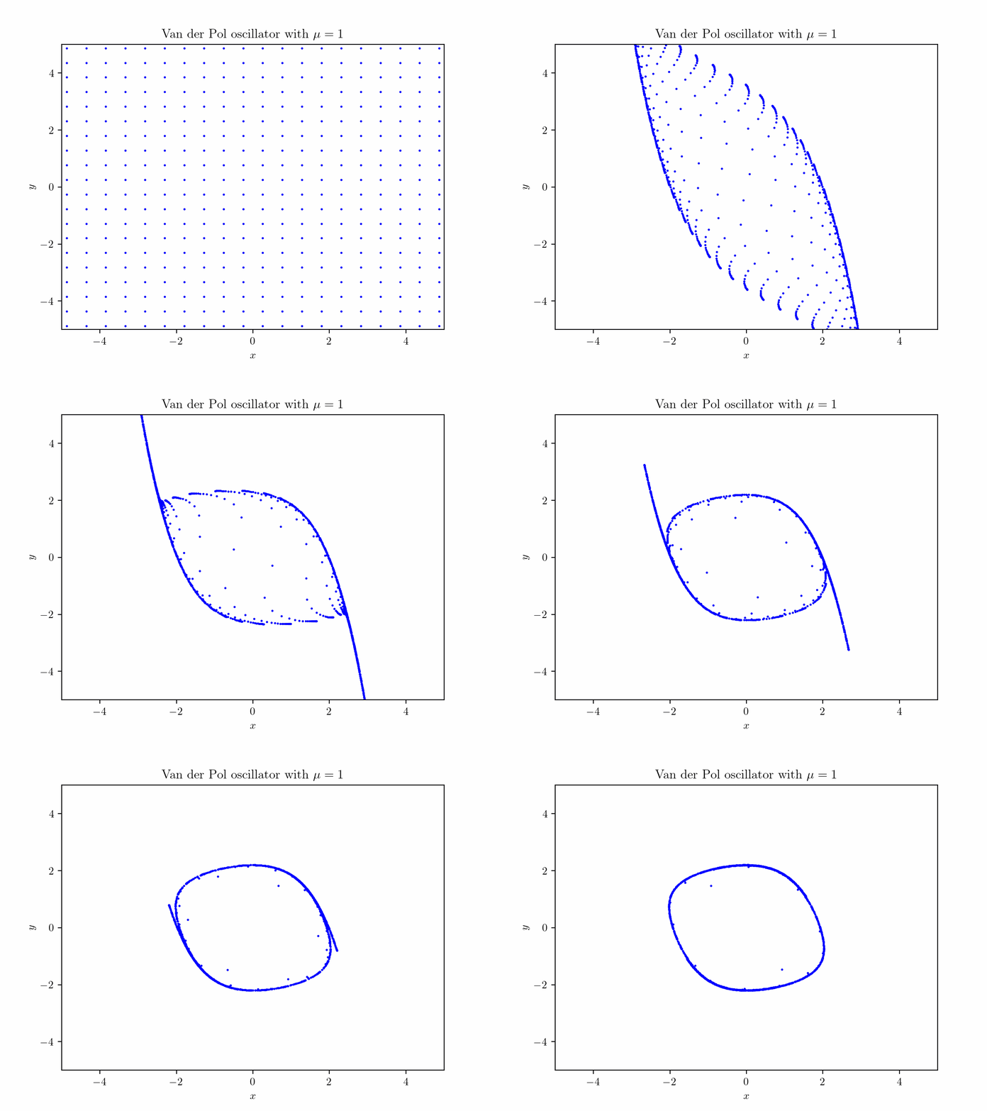
where $\mu$ is just a scalar value, which can be chosen arbitrarily. We will plot $x$ on the horizontal axis and $y$ on the vertical axis. This system is named after the Dutch electrical engineer Van der Pol, who was working with a simplified version of vacuum tubes in electrical circuits. I just want to look at the interesting behavior of this system to explore the usage of phase spaces (I basically saw this interesting image on Wikipedia, which shows a limit cycle). To illustrate this, consider a grid of many starting points - basically representing different starting conditions - then we start the time for all of these systems at once. This is what happens:
Animation created by Tobias Steinbrecher
Note that $x$ and $y$ are the coordinates in our phase space.
You might see that there is some kind of loop where many points end up on. This is also called a limit cycle. The concept of points in the phase space being attracted to certain sets of states is called attractors. The limit cycle in this case, is an example of an attractor.
There are many other attractors, which can even be classified in their behavior. Especially in the context of natural phenomena attractors are very intersting.
Lorenz attractor
The Lorenz attractor is another attractor and very famous because of its interesting behavior. The dynamical system has three degrees of freedom and consists of the following differential equations:
where $\sigma, \rho, \beta$ are the systems parameters. The meteorologist Edward Lorenz was studying the behavior of weather systems, which led him to a mathematical model of atmospheric convection, described by the three differential equations above.
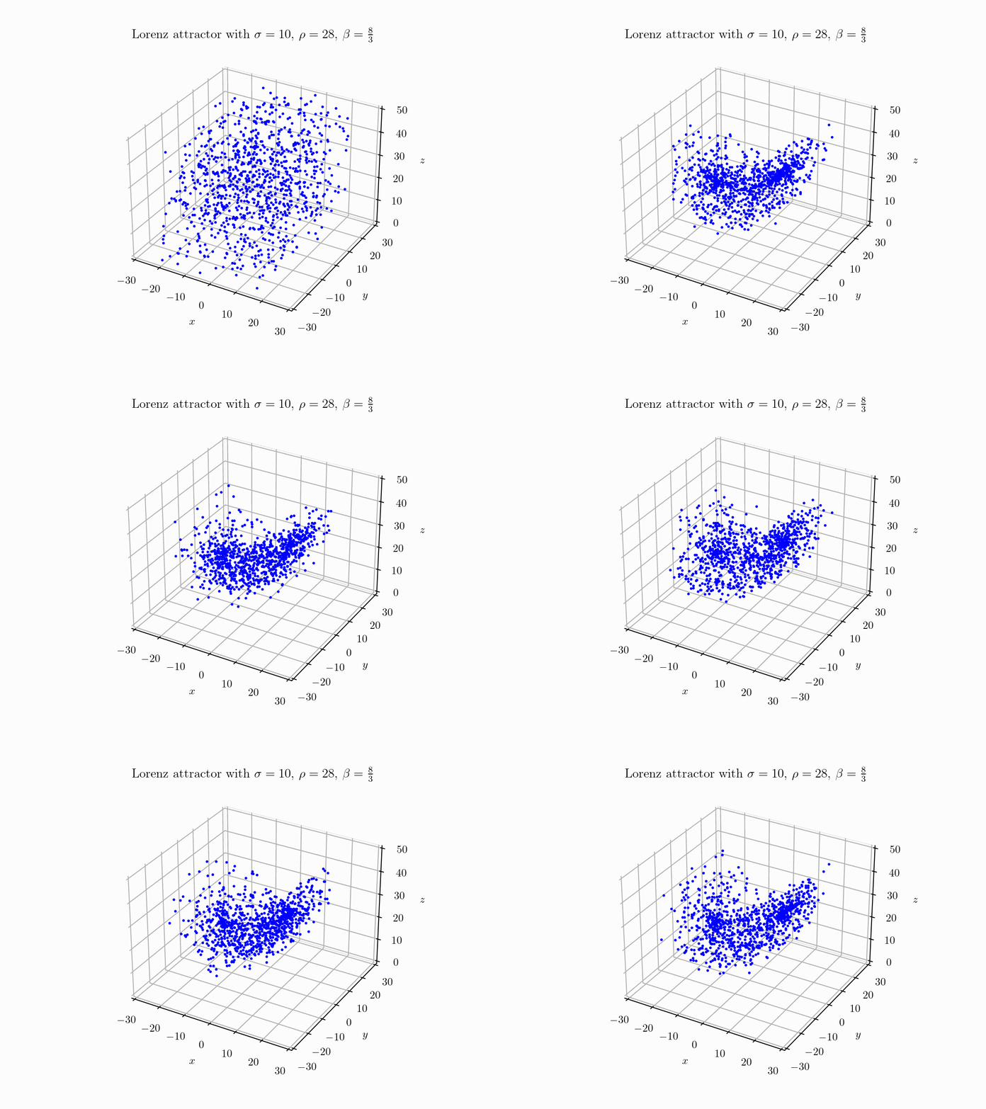
As we are just interested in the behavior of the system, we could go ahead and do the same thing we did for the Van der Pol oscillator: choose system parameters, plot some points in phase space (1000 in this case, drawn from uniform distribution) and watch them evolve over time:
Animation created by Tobias Steinbrecher
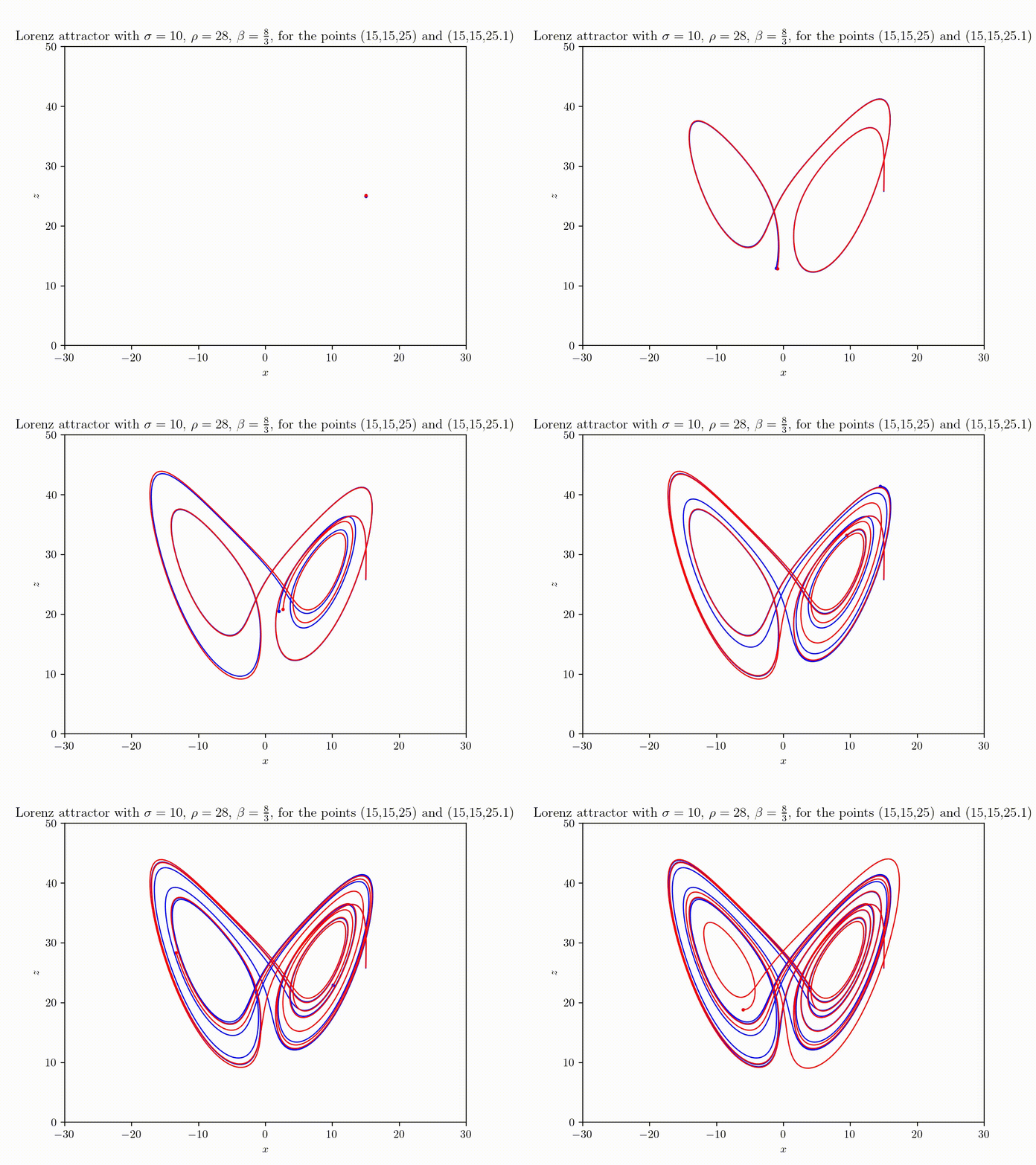
Note that in this case we have a three-dimensional phase space. The situation seems quite messy, but one can clearly detect something like two disks forming. To investigate further it might be necesarry to plot the real trajectories of fewer points. Additionally we will only consider the $xz$-plane. I created the following animation:
Animation created by Tobias Steinbrecher
In the above animation one can see another very interesting behavior. The trajectories of two very close points with an initial distance of $0.1$ diverge over time. This interesting behavior is also known as chaos. The current description of chaos seems kind of superficial and empirical. To investigate further, what chaos really is, one might want to step back from the Lorenz attractor, which actually has many more interesting properties. The chaotic behavior of the Lorenz attractor or rather a weather system was also popularized as Butterfly effect. The aim of the rest of this article is to search for a better understanding of chaotic behavior of dynamical systems.
What is chaos?
First of all one should clarify what people understand when talking about chaos. In Introduction to the Modeling and Analysis of Complex Systems, Hiroki Sayama describes chaos with the following 5 properties:
- Chaos is a long-term behavior of a nonlinear dynamical system that never falls in any static or periodic trajectories.
- Chaos looks like a random fluctuation, but still occurs in completely deterministic, simple dynamical systems.
- Chaos exhibits sensitivity to initial conditions.
- Chaos occurs when the period of the trajectory of the systems state diverges to infinity.
- Chaos occurs when no periodic trajectories are stable.
I am not quite satisfied with that kind of definition because it provides no rigorous mathematical frame to chaos.
Logisitc Map
A much simpler chaotic system is the logistic map. It was actually suggested to be used as a pseudo-random number generator in early computers. We can think of some population which is parametrized by some parameter $r$. Now we basically simulate the population over discrete time steps using some recurrence relation. Let $x_n$ be some measure of the population size in the $n$-th year or whatever time-unit one may use.
The difference between time-discrete and time-continuous dynamical systems was already pointed out above. We can build a model which describes the population size with a time-discrete model:
This recurrence relation can model reproduction and starvation, while $0 \leq x_n \leq 1$ describes the ratio of the population size and the maximum possible population size. Mathematically it’s basically a very simple polynomial of degree 2 with the parameter $r$, applied over and over again. With $x_0 = 0.5$ and $r=2$ we would obtain:
| $n$ (Year) | $x_n$ |
|---|---|
| $0$ | $0.5$ |
| $1$ | $2 \cdot 0.5 \cdot (1-0.5) = 0.75$ |
| $2$ | $2 \cdot 0.75 \cdot (1-0.75) = 0.5625$ |
| $3$ | $2 \cdot 0.5625 \cdot (1- 0.5625) \approx 0.7383 $ |
| $4$ | $2 \cdot 0.7383 \cdot (1- 0.7383) \approx 0.5797 $ |
For a more general case of an iterated function $f(f(f…(f(x_0))))$ the notation $f^N(x_0)$ such that $f^N(x_0) = x_n$ is used.
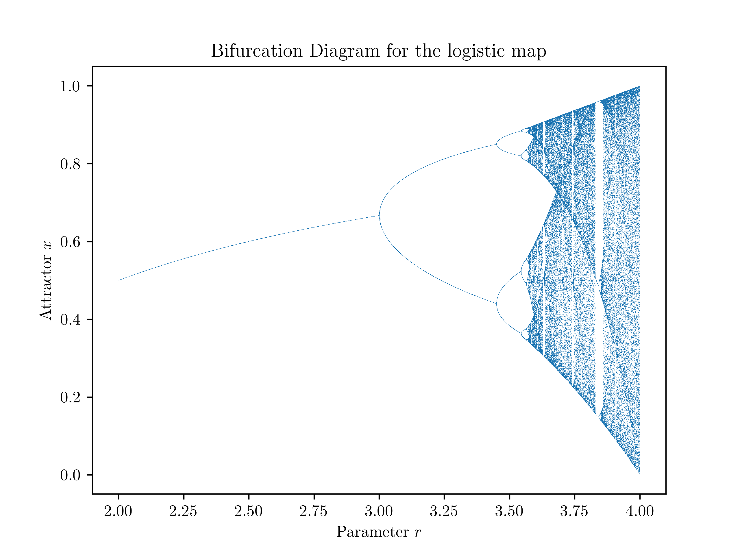
There are many very interesting things, which can be observed here. While for some values of $r$ the population size converges, for other values there seems to be periodic behavior. However, for bigger values (like $4$ for example - try it out yourself) there isn’t even a periodic behavior. It seems to be plausible to call this behavior chaotic. Note, that this convergence behavior is independant of the starting value $x_0$ and only depends on the parameter $r$. We could again use the term attractor for these observations. The attractors are varying in dependance of $r$. To get an insight in the actual dependence, lets plot the attractor values for the different values of $r$. We can basically do this, by picking many random points, in a range of interest, and then apply the iterated function:
Created by Tobias Steinbrecher
This type of diagram is also called bifurcation diagram, because one can clearly see these characteristic forking points (e.g. $r=3$) - bifurcations. It seems like there are some intervals for which there is complete choas and some other areas for which there is some kind of stability. There are so many more things which seem super interesting. You might want to read the Wikipedia-Article about the logisitic map. I am still looking for some clarification on how to more or less mearsure the chaotic behavior.
Lyapunov-Exponent
The Lyapunov-Exponent of a a dynamical system, describes a possibility to measure how fast two very close points in phase space diverge or converge. Let $x_0$ be starting point in one dimensional phase space and $\varepsilon$ an infinitesimal small change to these starting conditions. We could try to measure how quickly this small change $\varepsilon$ increases, thus, how quickly the distance $|f^N(x_0)-f^N(x_0+\varepsilon)|$ between the two trajectories increases. We assume that the distance change over time can be approximated by an exponential function, such that it diverges or converges exponentially. The exponent $\lambda$ is refered to as the Lyapunov-Exponent:
If we apply the infinitesimal size of $\varepsilon$ and let $N\to \infty$, we get:
Actually, when we let $\varepsilon \to 0$, we get the derivative of $f^N$ with respect to $x$ at the point $x_0$, which will be denoted in Lagrange-Notation ($f’(x_0)$):
As we iterate the function an infinite number of times, which is nothing else than plugging the current value in the function over and over again, while updating it, we can apply the chain rule to simplify the $f’^N$-Term. The chain rule gives us:
So we get a product of the different steps:
Additionally we can apply simple logarithm rules ($\log(a\cdot b) = \log(a) + \log(b)$) to convert the product into a sum, such that we get:
So if we have some amount (big amount) of starting points, we could actually calculate $\lambda$. What what does $\lambda$ mean?
If we look back at the assumption we made (exponential behavior of distance over time): $\delta \approx \varepsilon e^{\lambda N}$ We can conclude the following significance of $\lambda$:
- $\lambda > 0$: this means, that the infinitesimal starting distance will grow exponentially over time.
- $\lambda < 0$: this means, that the distance won’t grow indefinitely and converge.
We would expect case 2. intervals where we observed more or less stable behavior. By writing a little programm, which calculates these exponents and plots them, we can check our guess (Actually the other visualizations also required programming - but in this case I want to emphasize the use of computers): But first we need to get the first derivative of $f$, which should be no problem:
When using the formula derived above, we can create the following diagram:
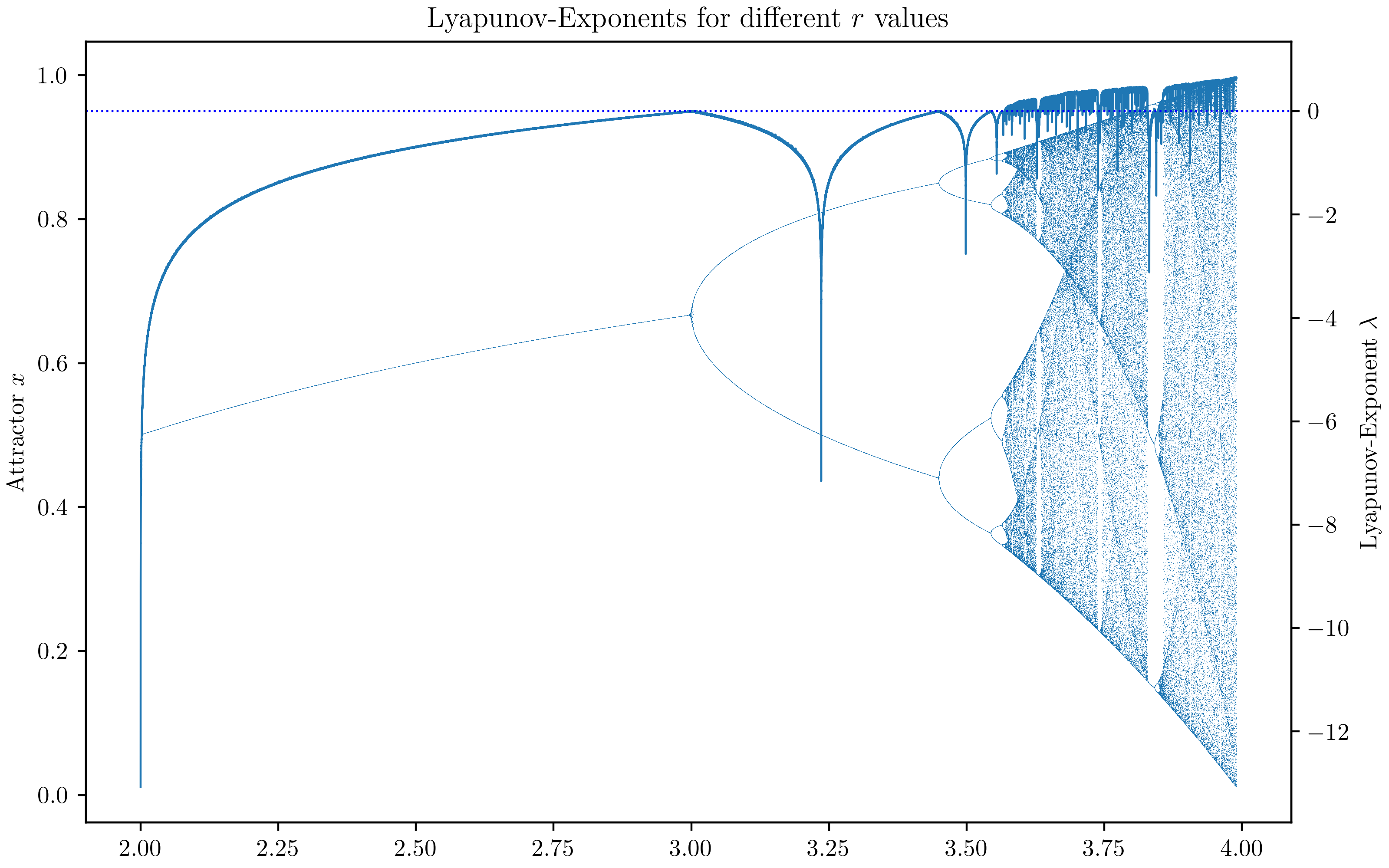
Created by Tobias Steinbrecher
One can see how the value of $\lambda$ is bigger than $0$ in the regions of chaos and how it’s dropping below $0$ in the intervals of stability. By examining the Lyapunov exponents in the diagram, we can gain a deeper understanding of the logistic maps behavior and the range of dynamics it can exhibit. This information contributes to our understanding of nonlinear systems and their sensitivity to initial conditions.